Excel 2016中设置单元格下拉列表的相关教程介绍

Excel办公软件是我们平时工作生活中用来处理数据、统计分析的，使用非常广泛。excel2016和之前的2010版在功能上是有一些不同的，其中给单元格设置下拉选项，在2010版本中的数据有效性里面可以设置，但是2016版本的excel没有数据有效性这个图标了，那该怎么办呢？本文主要是详细介绍在Excel 2016中如何给单元格设置下拉选项。
Excel 2016中如何给单元格设置下拉列表选项？
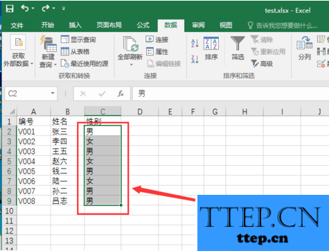
1、打开一个excel表，选中需要设置下拉选项的区域；

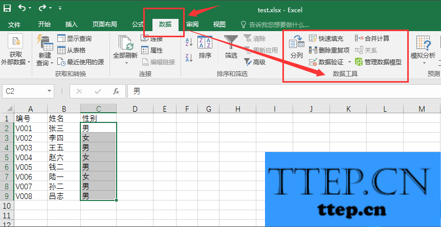
2、在Excel表的菜单选项中找到“数据”，数据菜单下方的工具栏中找到“数据工具”板块；

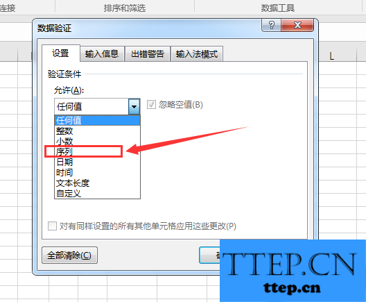
3、点击数据工具选项里的“数据验证”右边的倒三角，找到“数据验证”图标；

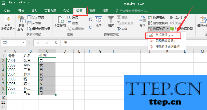
4、点击“数据验证”图标，弹出数据（了解更多excel教程资讯，访问wmzhe---）验证设置框；

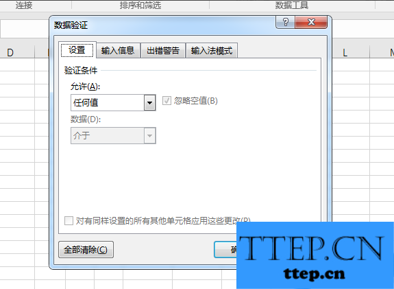
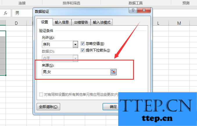
5、验证条件选择“序列”，来源里输入要设置的下拉选项，用英文状态下的逗号隔开；


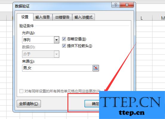
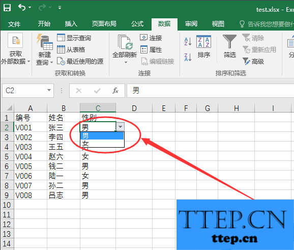
6、点击“确定”，之后可以在原数据表中看到想要的效果。